Overview
CPM is a DSM-based numerical approach for predicting and analysing how changes are likely to propagate through a system. The design of the system is decomposed into its components and the dependencies between them are captured and quantified. As a result, a product design is modelled as a DSM (and a corresponding numeric network), where the DSM-elements (nodes) represent the components or subsystems and the DSM-links (edges) their dependencies. Likelihood and impact values inside the DSM-cells (on the edges) represent the strength of the linkages with regard to propagation of engineering changes. Afterwards, a stochastic algorithm is applied to calculate the combined risk of change propagation between components considering multiple steps of direct and indirect change propagation. Based on this product model and the combined risk values, CPM generates different diagrams (i.e. Change Propagation Tree, In/Out Risk Portfolio, etc.) to support change propagation analysis.
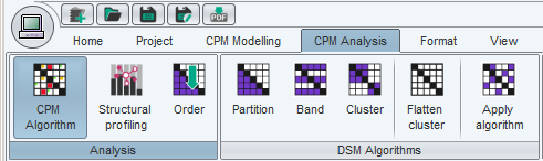
This algorithm can be applied using the 'CPM algorithm' button in the 'Analysis' band on the 'CPM Analysis' tab.
Steps to create a CPM simulation
Typically the following process is followed to create an CPM simulation (see below for practical hints and tips):
1. Create a system linkage model must be created. This captures the elements (e.g. components of a product) of the system and the direct linkages between elements. The model is further elaborated into a probabilistic model that captures the likelihood and impact of a change propagating between each connected pair of elements.
2. Apply CPM algorithm to the probabilistic system linkage model in order to compute combined likelihoods, impacts and risks. The calculations compute the probabilistic “combined” values over all potential propagation paths between each element pair, thus accounting for direct and indirect connection.
- To execute CPM algorithm, first open the worksheet you wish to simulate. Then,Click the 'CPM algorithm' button in the 'Analysis' band on the 'CPM Analysis' tab. A dialog will appear where user is given following options.Select whether to apply the algorthim on the whole matrix or a selection
- Path length (This determines the change propagation path lenth. Data processing times relate exponentially with path length. So a practical limit of three or four steps is suggested.)
- Specifying multiple initiating components( if required). By default, CPM produces a general risk profile considering single changes – one at a time – to each component. However, if multiple components change simultaneously, they can be selected accordingly to produce a specific change profile.
3. A new CPM model will be created as a result of the analysis with combined likelihood and impact values, as calculated in the previous step. The consequences of a change request are determined by analysing this model, through a variety of tabular and graphical representations.
Setting up CAM for distributed computing
CAM supports distributed computing for simulation experiments. This facilitates large, computationally-expensive experiments that otherwise would not be possible. (Note this feature does not currently support standard CPM simulations, only simulation experiments)
It is quite easy to set up:
How to set up a simulation cluster
To set up a simulation cluster, you must decide which computers will be 'servers' (ie, will run simulations) and which will be the client (ie., that you will use to configure and manage simulation jobs). Simulation jobs are co-ordinated via files in a shared folder. All the computers that participate must therefore have (read and write) access to the same shared folder. It is not intended for remote shared folders, because the protocol requires frequent file read and write operations.
On each computer that you wish to be a server:
- Make sure that the toolboxes and palettes for the simulation you wish to distribute are installed
- Start CAM normally
- Under the 'Tools' menu, select the option 'Start simulation server'.
- Enter the name of the shared folder (as visible to that computer).
- Press the 'start server' button.
How to distribute simulation experiments over a cluster
- On the client machine, push the button 'distribute over cluster' which appears after configuring and starting a simulation experiment.
- A dialog will appear, allowing you to enter the path to the shared folder (as visible to to the client machine) and discover available servers.
- After clicking the 'Distribute job' button, the progress dialog will be altered to allows the progress of all machines in the cluster to be monitored. Note it may take some seconds for the distributed job to start up.
Notes:
- All computers must run the same version of CAM, including the same palettes and plugins.
- The distributed computing carries a significant setup overhead. It is only worthwhile to distribute an experiment that takes several minutes or more.
- All computers will use almost all their processor power to run simulations, and cannot be used for other tasks at the same time.
- All simulation data will be lost if any server or the client is interrupted, runs out of memory, etc, while running a distributed job.
- The CAM server applications will occasionally need restarting between jobs, for instance if a job is interrupted. Do this when a server no longer appears to respond when viewed from the client machine.